
Time Series Analysis Baby Steps Using R
This tutorial consists of my baby steps towards time series analysis. I will provide lots of supporting links, along with this tutorial, that helped me a lot to get a grip on this topic.
First thing first, What is “Time Series”?
Sequence of measurements/observations of the same variable over time.
Examples of Time Series can be:
- Daily closing price of a particular stock for last 1 year
- Yearly number of computer science graduates for the last 5 years
All right, then, what is “Time Series Analysis”?
The aims of time series analysis are to describe and summarize time series data, fit low-dimensional models, and make forecasts.
In simple words, what I understood, we have to understand the nature of time series data then fit it into a model to forecast.
Lets get our hands dirty and do some fun. The data set I am going to use is the “Nile River Flow” data set which is available in this link.
Open you R-Studio (as I am going to use R-Studio), create a new R Script and put the following code to read the “Nile River Flow” data set.
# read csv file
NileData <- read.csv(file.choose(),header=TRUE,sep=",")
head(NileData)
in the console you are going to see the following values:
X time Nile
1 1871 1120
2 1872 1160
3 1873 963
4 1874 1210
5 1875 1160
6 1876 1160
The first is the serial, second is the time(year for this case) and last column represents the value of the river flow on that year.
Now, lets convert this data to time series object. You can check the details for ts function from this link.
# convert to time series object
NileTimeSeriesObject <- ts(NileData[,3], frequency=1, start=c(1871,1))
plot.ts(NileTimeSeriesObject)
output will look like the following:
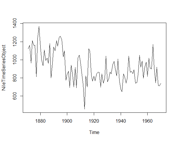
Prior to building a model we should check whether the data is stationary or not as we can not build model for time series until and unless it is stationary. If the data is not stationary, first we should transform it to stationary data using Differencing, Detrending etc.
So, A series xt is said to be stationary if it satisfies the following properties:
- The mean E(xt) is the same for all t.
- The variance of xt is the same for all t.
- The covariance (and also correlation) between xt and xt-h is the same for all t.
Please check the details about stationary and non-stationary data from this link and how to calculate mean, variance and standard deviation from this link.
We can identify this by simple looking at the timeseries plot above figure or with help of the “Augmented Dickey-Fuller Test” using the following code to check whether the series is stationary enough or time series modeling or not.
> adf = adf.test(NileTimeSeriesObject)
> adf

	Augmented Dickey-Fuller Test

data:  NileTimeSeriesObject
Dickey-Fuller = -3.3657, Lag order = 4, p-value = 0.0642
alternative hypothesis: stationary
Though it shows our data is stationary but if we try to fit in a line we will notice the mean is not constant over time. The lm() function used to fit linear model.
plot.ts(NileTimeSeriesObject)
abline(reg=lm(NileTimeSeriesObject~time(NileTimeSeriesObject)))

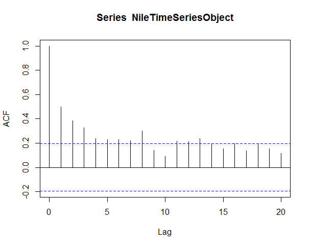
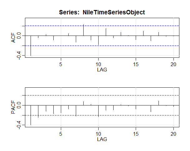
We can also use Auto Correlation Function (ACF) to determine the stationarity of our data set.This is a widely used tool in time series analysis to determine stationarity and seasonality.
acf(NileTimeSeriesObject,lag.max = 20)
This line of code will give us output some thing like this, please note that the ACF should show exponential decay for stationary series data
we can use differencing to make out series more stationary with the following code. I found this link useful about the diff function.
NileTimeSeriesObject<-diff(NileTimeSeriesObject)
plot.ts(NileTimeSeriesObject)
abline(reg=lm(NileTimeSeriesObject~time(NileTimeSeriesObject)))
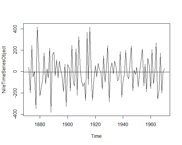
Now it looks good, what you say? check details about stationarity and differencing from this link.
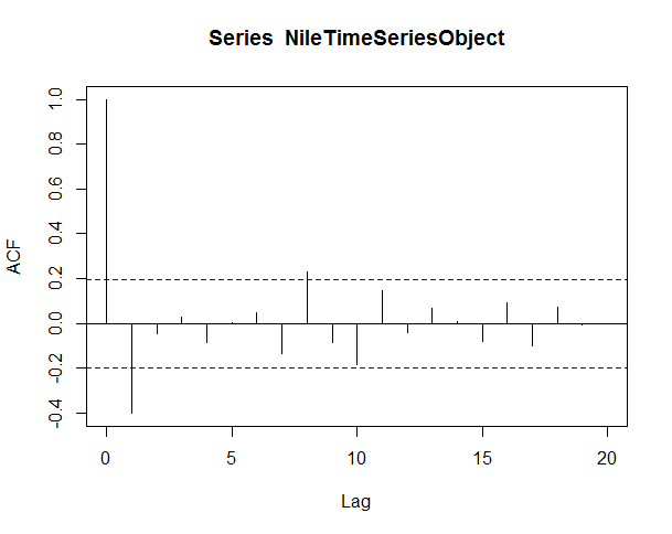
As all significant correlation being removed after lag 1 it is time to fit a time series model to the data using Autoregressive Integrated Moving Average(ARIMA) model.
Why ARIMA? Why not Exponential Smoothing?
The best answer I got:
While exponential smoothing methods are useful for forecasting, they make no assumptions about the correlations between successive values of the time series. We can sometimes make better models by utilizing these correlations in the data, using
Autoregressive Integrated Moving Average (ARIMA)models.
The arima function takes in 3 parameters (p,d,q), which correspond to the Auto-Regressive order, degree of differencing, and Moving-Average order.
To select the best ARIMA model we will inspect the Auto Correlation Function(ACF) and Partial Auto Correlation Function (PACF).
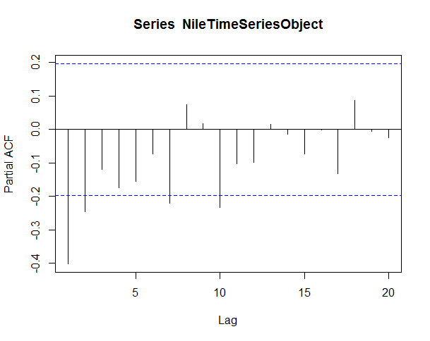
The ACF/PACF plot give us suggestions on what degree of parameters to utilize.
Identification of an AR model is often best done with the PACF.
Identification of an MA model is often best done with the ACF rather than the PACF.
The two most basic rules are:
- If the ACF is a sharp cutoff the
qcomponent is equal to the last significant lag. This type of model also often has a PACF with a tapering pattern. - If the PACF has a sharp cutoff, the
pcomponent is equal to the last number of significant lags. Again, the ACF may exhibit a tapering pattern.
Now we can test the following two models first based on the basic rules mentioned earlier
arima(NileTimeSeriesObject, order=c(0, 1, 2))
arima(NileTimeSeriesObject, order=c(7, 1, 0))
> arima(NileTimeSeriesObject, order=c(0, 1, 2))

Call:
arima(x = NileTimeSeriesObject, order = c(0, 1, 2))

Coefficients:
          ma1     ma2
      -1.7092  0.7092
s.e.   0.1277  0.1256

sigma^2 estimated as 20702:  log likelihood = -629.87,  aic = 1265.75
> arima(NileTimeSeriesObject, order=c(7, 1, 0))

Call:
arima(x = NileTimeSeriesObject, order = c(7, 1, 0))

Coefficients:
          ar1      ar2      ar3      ar4      ar5      ar6      ar7
      -1.2995  -1.3533  -1.2250  -1.0675  -0.8658  -0.5946  -0.3906
s.e.   0.0934   0.1515   0.1843   0.1921   0.1843   0.1581   0.0996

sigma^2 estimated as 24030:  log likelihood = -634.94,  aic = 1285.87
The Akaike Information Critera (AIC) is a widely used measure of a statistical model. It basically quantifies 1) the goodness of fit, and 2) the simplicity/parsimony, of the model into a single statistic. When comparing two models, the one with the lower AIC is generally “better”.
The first model arima(NileTimeSeriesObject, order=c(0, 1, 2)) gives AIC value 1265.75 and the second model arima(NileTimeSeriesObject, order=c(7, 1, 0)) gives AIC value 1285.87.
So, we can say that arima(NileTimeSeriesObject, order=c(0, 1, 2)) is the best fitted model. We can test our findings using the auto.arima() function.
> auto.arima(NileTimeSeriesObject)
Series: NileTimeSeriesObject
ARIMA(1,0,1) with zero mean

Coefficients:
         ar1      ma1
      0.2544  -0.8741
s.e.  0.1194   0.0605

sigma^2 estimated as 20177:  log likelihood=-630.63
AIC=1267.25   AICc=1267.51   BIC=1275.04
auto.arima() function gives AIC value 1267.25 so it is evident that arima(NileTimeSeriesObject, order=c(0, 1, 2)) is the best fitted model for our data set.
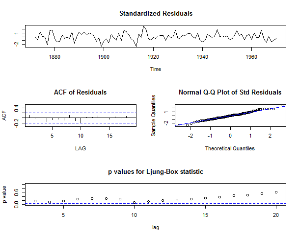
If we plot the residuals we will see all the spikes are now within the significance limits, and so the residuals appear to be white noise.
To know more about Residual Diagnostics please check this link and to understand White Noise please check this link.
res <- residuals(Niletimeseriesarima)
library("forecast")
tsdisplay(res)
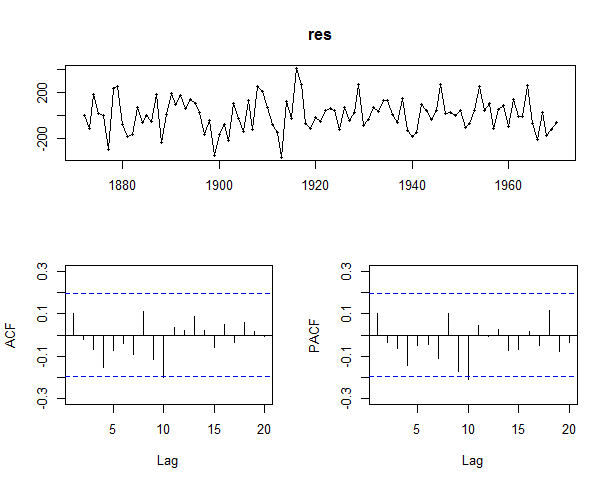
A Ljung-Box test also shows that the residuals have no remaining autocorrelations.
> Box.test(Niletimeseriesarima$residuals, lag=20, type="Ljung-Box")

	Box-Ljung test

data:  Niletimeseriesarima$residuals
X-squared = 15.537, df = 20, p-value = 0.7449
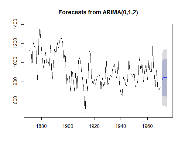
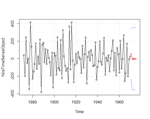
As we have found our best fitted model for our data set, lets forecast for next 5 years and plot the result using the following command.
> fit1forecast <- forecast.Arima(arima(NileTimeSeriesObject, order=c(0, 1, 2)), h=5)
> fit1forecast
     Point Forecast    Lo 80    Hi 80    Lo 95    Hi 95
1971       820.3071 639.4648 1001.150 543.7326 1096.882
1972       836.0617 644.0816 1028.042 542.4535 1129.670
1973       836.0617 641.2674 1030.856 538.1495 1133.974
1974       836.0617 638.4932 1033.630 533.9067 1138.217
1975       836.0617 635.7574 1036.366 529.7227 1142.401
> plot.forecast(fit1forecast)
I found another R package astsa gives a better view for arima modeling. The following commands can be used for arima modeling and forecasting.
#insall and load astsa package
install.packages("astsa")
library("astsa")
acf2(NileTimeSeriesObject,max.lag=20)
> sarima(NileTimeSeriesObject, 0, 1, 2)
initial  value 5.640106
iter   2 value 5.311943
iter   3 value 5.119169
iter   4 value 5.118704
iter   5 value 5.116513
iter   6 value 5.113400
iter   7 value 5.046436
iter   8 value 5.021747
iter   9 value 5.021601
iter  10 value 5.021592
iter  11 value 5.021422
iter  12 value 5.021397
iter  13 value 5.021395
iter  14 value 5.021394
iter  14 value 5.021394
iter  14 value 5.021394
final  value 5.021394
converged
initial  value 5.025353
iter   2 value 5.023444
iter   3 value 5.020315
iter   4 value 5.019311
iter   5 value 5.011232
iter   6 value 5.009947
iter   7 value 5.008000
iter   8 value 5.007893
iter   9 value 5.007884
iter  10 value 5.007863
iter  11 value 5.007850
iter  11 value 5.007850
iter  11 value 5.007850
final  value 5.007850
converged
$fit

Call:
stats::arima(x = xdata, order = c(p, d, q), seasonal = list(order = c(P, D,
    Q), period = S), xreg = constant, optim.control = list(trace = trc, REPORT = 1,
    reltol = tol))

Coefficients:
          ma1     ma2  constant
      -1.7218  0.7218    0.0496
s.e.   0.1391  0.1375    0.1585

sigma^2 estimated as 20656:  log likelihood = -629.83,  aic = 1267.65

$degrees_of_freedom
[1] 96

$ttable
         Estimate     SE  t.value p.value
ma1       -1.7218 0.1391 -12.3743   0.000
ma2        0.7218 0.1375   5.2504   0.000
constant   0.0496 0.1585   0.3129   0.755

$AIC
[1] 10.99638

$AICc
[1] 11.02088

$BIC
[1] 10.07502
sarima.for(NileTimeSeriesObject,5,0,1,2)
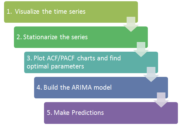
To conclude, the flow chart for Time Series Analysis is like the following (taken from http://www.analyticsvidhya.com).
And the complete version of my R Scripts are as follows:
library("forecast")

# read csv file and check summary
NileData <- read.csv(file.choose(),header=TRUE,sep=",")
head(NileData)
summary(NileData)

# convert to time series object
NileTimeSeriesObject <- ts(NileData[,3], frequency=1, start=c(1871,1))
plot.ts(NileTimeSeriesObject)
abline(reg=lm(NileTimeSeriesObject~time(NileTimeSeriesObject)))

acf(NileTimeSeriesObject,lag.max = 20)
pacf(NileTimeSeriesObject, lag.max=20)

# adf test to check data set is stationarize enough or not
adf = adf.test(NileTimeSeriesObject)
adf

# differencing the data set to stationarize
diffNileTimeSeriesObject<-diff(NileTimeSeriesObject)
plot.ts(diffNileTimeSeriesObject)
abline(reg=lm(diffNileTimeSeriesObject~time(diffNileTimeSeriesObject)))

acf(diffNileTimeSeriesObject,lag.max = 20)
pacf(diffNileTimeSeriesObject, lag.max=20)

# find the best fitted model based on acf and pacf
fit1 <- arima(diffNileTimeSeriesObject, order=c(0, 1, 2))
fit1

fit2 <- arima(diffNileTimeSeriesObject, order=c(7, 1, 0))
fit2

# test the model
auto.arima(diffNileTimeSeriesObject)

# residuals diagnostics
res <- residuals(fit1)
tsdisplay(res)

Box.test(res, lag=20, type="Ljung-Box")

#forecast
fit1forecast <- forecast.Arima(arima(NileTimeSeriesObject, order=c(0, 1, 2)), h=5)
fit1forecast
plot.forecast(fit1forecast)


#insall and load astsa package
#install.packages("astsa")
library("astsa")
acf2(diffNileTimeSeriesObject,max.lag=20)
sarima(diffNileTimeSeriesObject, 0, 1, 2)
#sarima(diffNileTimeSeriesObject, 7, 1, 0)
sarima.for(diffNileTimeSeriesObject,5,0,1,2)
Md Shiefuzzaman • September 1, 2016